

A matrix may have thousands of columns while much of its variation follows only a few patterns. Photographs contain repeated shapes, and measured variables often change together. A low-rank approximation represents this shared structure through a small set of directions and the weights needed to combine them.
rsvd computes these approximations for dimension reduction, compression, and data analysis. It uses random combinations of the input to find a small subspace, then performs the main factorization within that subspace. This can reduce the work when the requested rank is small relative to the matrix dimensions and the singular values decay.
The package provides several matrix decompositions, principal component analysis, and robust principal component analysis, together with plotting functions. It accepts ordinary R matrices and supports sparse matrices from the Matrix package. Randomized principal component analysis can center and scale sparse input implicitly, avoiding a dense copy of the processed data. The package paper describes the algorithms and their applications.
install.packages("rsvd")

# Development version:
# install.packages("remotes")
# remotes::install_github("erichson/rSVD")
This source is the 2.0.0 release candidate; the CRAN badge shows the
published version. It requires R 4.4 or later and Matrix 1.7-0 or later.
The minimum R version follows the Matrix dependency. CI also tests newer
R releases alongside the R 4.4 series. Sparse dispatch works without
attaching Matrix with library(Matrix).
This example makes a matrix from three underlying patterns, then adds small measurement noise. Asking for rank three retains the shared patterns while leaving a residual. The example is small enough to inspect; the later benchmarks show where the randomized calculation saves time.
library(rsvd)
set.seed(42)
patterns <- matrix(rnorm(120 * 3), 120, 3)
weights <- matrix(rnorm(3 * 80), 3, 80)
A <- patterns %*% weights + 0.01 * matrix(rnorm(120 * 80), 120, 80)

fit <- rsvd(A, k = 3)
A_approx <- tcrossprod(sweep(fit$u, 2, fit$d, "*"), fit$v)
norm(A - A_approx, "F") / norm(A, "F")
The last expression is the relative reconstruction error. It compares
the size of the residual with the size of the original matrix. Keep
fit when you need a compact representation;
A_approx allocates a full matrix again. Use
rpca() when columns should be centered or scaled before
finding the directions. rsvd() uses the supplied values as
they are.
Choose the factors that the analysis needs. An SVD gives orthogonal directions, ID and CUR retain actual columns or rows, and robust PCA estimates a separate sparse corruption component.
| Function | Result and typical use |
|---|---|
rsvd(A, k) |
Leading singular vectors and values for low-rank compression. |
rpca(A, k) |
Principal loadings, component variances, and optional scores. |
rqb(A, k) |
An orthonormal basis Q and a compressed matrix B. The randomized basis includes oversampling. |
rid(A, k) |
Selected columns and interpolation coefficients; row ID is also available. |
rcur(A, k) |
Selected columns, selected rows, and their connector matrix. |
rrpca(A) |
A low-rank component and an entrywise sparse corruption component. |
Consider a matrix whose columns are measurements, images, or time series. Its rank is the number of independent directions spanned by those columns. If every column can be assembled from ten underlying patterns, the matrix has rank at most ten, regardless of how many columns it contains. A factorization stores the patterns and the coefficients that reconstruct each column from them.
Measured data rarely have exactly low rank. Noise may make a matrix full rank even when most of its variation follows a few patterns. A low-rank approximation retains those patterns and leaves a residual, the difference between the data and their reconstruction. Working with the approximation can reduce storage and simplify later calculations or visualization. The application determines which residual is acceptable; rank alone cannot distinguish noise from a weak but useful signal.
The singular value decomposition (SVD) gives orthogonal directions
for representing this variation. Keeping the leading k
terms gives
A \approx U_k D_k V_k^{T}.The columns of U and V are orthonormal left and right directions,
respectively, and D is diagonal. Its nonnegative entries are the
singular values, ordered from largest to smallest. Each left direction,
right direction, and singular value defines one rank-one pattern. The
squared singular value measures that pattern’s contribution to the
squared Frobenius norm, so the leading terms retain the strongest
variation first. The exact truncated SVD minimizes the Frobenius error
among rank-k approximations. Randomized SVD aims to
approach this accuracy while reducing the cost of finding the
directions.
The equations here use real matrices, for which superscript T denotes transpose. With complex input, reconstruction uses H, the conjugate transpose, which also conjugates the matrix entries. rsvd supports complex matrices; the reconstruction code must use the corresponding transpose.
An image makes the role of these patterns visible. A grayscale image is a matrix of pixel intensities. Its leading SVD terms capture broad shapes and repeated features, while additional terms recover finer detail. The bundled tiger image lets us compare the original pixels with reconstructions at different ranks.
library(rsvd)
data(tiger)

set.seed(42)
fit <- rsvd(tiger, k = 150)

# Keep fit$u, fit$d, and fit$v for a compact representation.
# Reconstruct only when a dense image is needed; avoid an explicit diag(fit$d).
tiger_approx <- tcrossprod(sweep(fit$u, 2, fit$d, "*"), fit$v)
norm(tiger - tiger_approx, "F") / norm(tiger, "F")
For complex data, reconstruct with
sweep(fit$u, 2, fit$d, "*") %*% Conj(t(fit$v)).
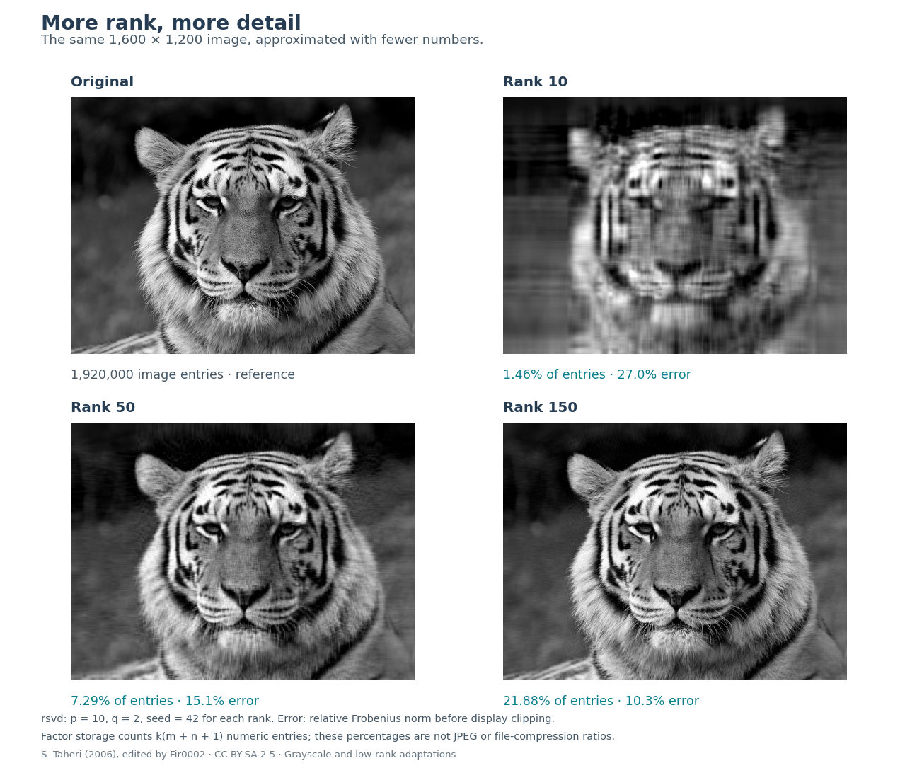
Increasing the rank improves the tiger reconstruction at the cost of larger factors. For this 1,600-by-1,200 image, rank 50 stores 7.3% of the original number of numeric entries and has 15.1% relative Frobenius error. Rank 150 stores 21.9% of the entries and reduces the error to 10.3%. The panels show the original image and reconstructions at ranks 10, 50, and 150.
An m-by-n matrix contains
m * n numbers. Its rank-k SVD factors contain
k * (m + n + 1), accounting for both sets of directions and
the singular values. These counts describe numeric storage in matrices
and factors; JPEG and PNG compression use different representations.
Reconstructing the image allocates the full dense matrix again, so
storing the factors preserves the compact representation.
Many calculations can use the factors directly. To multiply the
approximation by a vector, project the vector onto V, multiply the
resulting k coefficients by the singular values, and
combine the columns of U with those weights. The work grows with
k * (m + n) rather than m * n. This saving
applies to subsequent products as well as any saving obtained when
computing the factorization.
Image: S. Taheri (2006), edited by Fir0002, CC BY-SA 2.5, via Wikimedia Commons. The package supplies a grayscale version, and the panels add low-rank reconstructions. Reproduce this figure.
The tiger example shows how to use the factors. Computing them
efficiently starts with finding a subspace that captures most of the
input’s variation. Suppose A is a tall matrix with m rows
and n columns, and we want k dominant
directions. A random weighted combination of its columns contains
contributions from many directions at once. Directions with larger
singular values contribute more strongly, allowing a small collection of
these combinations to capture the dominant subspace.
The algorithm draws a random matrix called omega with n
rows and ell = min(k + p, m, n) columns. Its entries are
Gaussian by default. Up to p extra columns provide
oversampling, which helps capture directions near the truncation
boundary. Multiplying A by this random matrix forms a
sketch, and a thin QR factorization gives an
orthonormal basis Q for the sketch. The original data are then projected
onto that basis. The two matrix products are
Y = A\Omega, \qquad B = Q^{T}A.Y contains the random combinations, while B expresses the original
columns in the coordinates of Q. The product QB approximates A. Because
B has only ell rows, its SVD is much smaller than the
original problem. For a 20,000 × 6,000 input with
k = 40 and p = 10, B has size 50 ×
6,000, or 300,000 entries compared with 120 million in A. Q has
20,000 × 50 entries. Products with the input and the factorization
routines require additional workspace beyond these compressed
arrays.
The algorithm computes an ordinary SVD of B and retains its leading
k terms. Multiplying its left singular vectors by Q maps
them back to the original coordinates. Its right singular vectors can be
used directly, and its singular values approximate those of A. The
returned fit$d stores these values as a vector. Random
sampling therefore determines the subspace in which conventional
numerical linear algebra completes the factorization. Wide inputs are
handled through the conjugate-transposed problem.
When singular values decay slowly, a small initial sketch may miss
some directions near the chosen rank. Power iterations strengthen the
separation between dominant and trailing directions before the final
projection. With q iterations, the idealized sketch is
Y = (AA^{T})^q A\Omega.This operation raises each singular value to the power
2 * q + 1, giving larger values greater weight. The
implementation obtains this effect through successive products with A
and its transpose, with orthonormalization after each product. It avoids
forming either the matrix of cross-products or its power. Each added
iteration requires further passes over the input. The package paper
develops the method through worked examples, and the Halko–Martinsson–Tropp survey
gives its error analysis.
For a dense tall matrix, a full SVD requires work on the scale of
m * n^2. With a fixed number of power iterations, the main
randomized products cost on the scale of m * n * ell. Thin
QR and SVD calculations add work on the scale of
(m + n) * ell^2. A sketch much narrower than the input can
therefore reduce the total work substantially. The products also use
optimized BLAS routines. Small inputs and ranks near the full dimension
leave less room to recover the overhead of forming the sketch.
The algorithm still reads the input repeatedly. The default
q = 2 requires six products with A or its transpose,
including the final projection. Each product applies the matrix to a
small collection of vectors, and the subsequent factorization uses the
compressed result. Increasing q can improve the
approximation to the dominant subspace, at the cost of additional
products.
The main thin arrays grow with (m + n) * ell, while a
dense input occupies m * n entries. Sparse products can use
the stored entries of A, although the sketches and factors are generally
dense. Sparsity alone says little about approximation quality; a matrix
with many zeros may still require many directions. The sparse examples
below combine structure that admits a low-rank approximation with
computation that preserves sparse input. Their cumulative R allocation
measurements also include temporary objects, so they exceed the storage
needed for the final factors.
The same low-rank representation provides the main computation for principal component analysis (PCA). After centering the observations and optionally scaling the variables, the right singular vectors give the principal loadings. The left singular vectors, weighted by their singular values, give the fitted scores. Keeping a few score columns places each observation in a small set of coordinates that describes the dominant variation in the processed data.
The iris data provide a small example whose coordinates are easy to
interpret. The larger examples below measure computational performance.
Install ggplot2 to use the plotting helpers.
library(rsvd)
data(iris)
set.seed(42)
pca <- rpca(as.matrix(iris[, 1:4]), k = 2, center = TRUE, scale = TRUE)
ggbiplot(pca, groups = iris$Species, ellipse = FALSE,
         ind_labels = FALSE)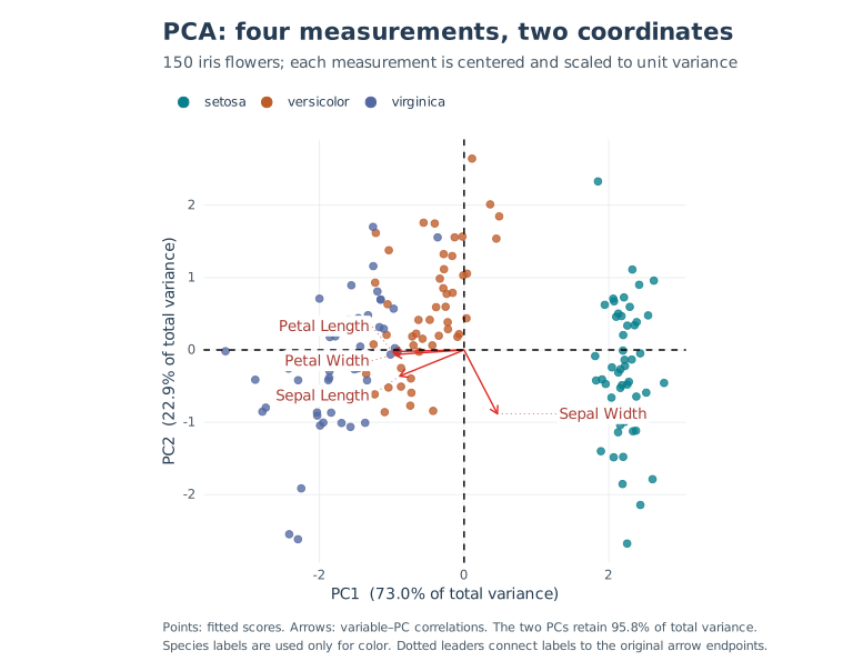
The first two components retain 95.8% of total variance in the centered, standardized iris measurements. Points are fitted flower scores, and arrows show variable–component correlations. The nearly parallel petal arrows indicate similar directions of variation. Species labels determine color and are excluded from fitting.
The figure adds a legend and separates variable labels for readability. Reproduce the styled figure and its numerical checks.
An SVD direction may combine every variable. When the original variables or observations have a useful interpretation, it can be preferable to express an approximation through actual columns or rows. An interpolative decomposition (ID) selects a subset of columns and uses them to reconstruct the others. For example, when columns are sensor measurements, their indices identify the sensors retained in the approximation. A column ID has the form
A \approx CZ.C contains k selected columns of A, and Z gives the
coefficients used to reconstruct every column from that subset. At the
selected indices, Z contains an identity matrix, so those columns
reproduce themselves. rid() returns C,
Z, and the column indices in idx. With
mode = "row", it selects rows in R and
reconstructs as Z %*% R.
CUR extends this idea by retaining both columns and rows. A small connector matrix U combines the columns in C with the rows in R,
A \approx CUR.For an observations-by-variables matrix, C contains actual variables
and R contains actual observations. Here U is a
k-by-k connector; the use of the letter U is
separate from its role as the left factor in an SVD. rcur()
returns C.idx and R.idx alongside the factors,
allowing the selections to be traced back to the data. Both ID and CUR
omit rows containing missing values with a warning. Returned row indices
then refer to the remaining complete observations.
In the tiger image, the selected columns and rows are strips of pixels. Their interpolation and connector factors reconstruct the full image from those strips.
set.seed(42)
id <- rid(tiger, k = 50)
id$idx[1:6]                     # Original column positions
tiger_id <- id$C %*% id$Z

set.seed(42)
cur <- rcur(tiger, k = 50)
tiger_cur <- cur$C %*% cur$U %*% cur$R

c(ID = norm(tiger - tiger_id, "F") / norm(tiger, "F"),
  CUR = norm(tiger - tiger_cur, "F") / norm(tiger, "F"))
Requiring factors to contain observed columns and rows restricts the possible approximations and usually sacrifices some accuracy relative to SVD. The selected columns need not be orthogonal, and different valid subsets can have different residuals. Selection also depends on the input’s units and scaling, since ID and CUR do not standardize variables automatically. The residual measures how well a subset reconstructs the data; the indices alone do not establish causal importance. The package paper describes the pivoted-QR constructions used by these routines.
The requested rank determines how much variation the approximation
can retain. A small k gives the largest computational
saving, but its adequacy depends on the application and the spectrum of
the input. For rsvd(A, k, p = 10, q = 2), the parameters
p and q control how accurately the algorithm
finds a subspace of that rank.
The nonnegative integer p adds sketch columns, up to the
matrix dimensions, to help capture the target subspace. The nonnegative
integer q adds power iterations. Increasing it can improve
accuracy for slowly decaying spectra, while requiring more passes over
the data. ID and CUR use q = 0 by default.
To separate the effect of rank from sampling error, first compare two
ranks with the same p and q. Then keep a rank
fixed and increase p or q. Increasing
k permits a richer approximation; increasing p
or q tries to find the chosen rank more accurately. A
similar residual after refining the sample suggests that the retained
rank, rather than the range finder, is limiting this reconstruction. Use
residuals and the needs of the later analysis to decide whether the
extra work is useful.
A useful reference for accuracy is the energy left outside the leading directions. Write Ak for the exact truncated SVD, and order the singular values of A from largest to smallest. Its squared Frobenius residual is
\|A-A_k\|_F^2 = \sum_{j>k}\sigma_j^2.The Frobenius norm is the square root of the sum of squared
magnitudes of the matrix entries. The equation says that the smallest
possible squared reconstruction error equals the sum of the squared
singular values discarded after the first k terms. A
full-rank matrix can therefore have a good low-rank approximation if
those trailing values are small. For a flat spectrum and a rank much
smaller than the dimensions, even the optimal approximation leaves a
large relative residual.
Tests and benchmarks compare reconstruction errors with this
truncation error and check orthogonality and subspaces. Exact recovery
is an appropriate expectation for an exact low-rank test matrix.
Individual singular vectors can change sign or complex phase, and
repeated singular values allow rotations within a subspace.
set.seed() controls sampling in a fixed numerical
environment; BLAS or package changes can still produce different
vectors.
Omitting k in rsvd() requests the full
available rank. This remains supported, including downstream uses such
as Procrustes alignment, but removes the computational advantage of a
small target rank. Base svd() is a natural reference for a
full deterministic SVD.
The recorded benchmarks examine how these savings appear at larger
matrix sizes, while comparing the same requested rank and returned
factors. The synthetic inputs contain low-rank signal plus noise.
Scaling cases run from 10,000 × 3,000 to 20,000 ×
6,000, and dense PCA, ID, and CUR use 15,000 ×
4,500 inputs. Measurements were made on Linux x86_64 with R
4.6.1, Matrix 1.7-6, and OpenBLAS 0.3.26 using four BLAS threads. They
were recorded on October 17, 2026, with source commit 421c803.
These saved measurements describe that implementation; they have not
been rerun for the later release-review fixes. Reported times are
medians of five calls after warmup, with method order rotated between
repetitions.
Tables pair deterministic / randomized measurements. Speedup is the deterministic median divided by the randomized median, calculated before rounding. A 10× speedup therefore means one tenth of the reference runtime. The figures show absolute costs alongside ratios to make the scale of each saving visible.
R allocations measure cumulative bytes allocated
during a separate profiled call, in GiB (2^30 bytes). This
quantity includes temporary R objects but does not measure peak resident
memory or live workspace, and it does not capture every allocation
inside native libraries. Input generation, explicit garbage collection,
and error calculations are excluded. Preprocessing and any required
sparse-to-dense conversion are included.
Relative error divides the Frobenius reconstruction residual by the Frobenius norm of the input, using the centered and scaled observations for PCA. The percentages report reconstruction error; explained variance uses a different quantity. The benchmark guide provides the fixtures, baseline calls, raw observations, environment, and commands needed to reproduce these results.
At rank 40, the measured SVD speedup increases from 24.2× to 45.3×
across the sizes in the table, with relative reconstruction errors close
to those of the deterministic reference. The comparison uses
base::svd(A, nu = k, nv = k) and rsvd() with
p = 10, q = 2. Base SVD computes the full singular spectrum
even when only k vectors are requested. This baseline
therefore measures the saving relative to a full SVD calculation; it
does not characterize every specialized truncated-SVD solver.
| Input | k | Time (s) | Speedup | R allocations (GiB) | Relative error |
|---|---|---|---|---|---|
| Dense, 10,000 × 3,000 | 40 | 16.858 / 0.697 | 24.2× | 1.234 / 0.133 | 9.67% / 9.68% |
| Dense, 20,000 × 6,000 | 40 | 97.157 / 2.144 | 45.3× | 4.928 / 0.267 | 9.67% / 9.68% |
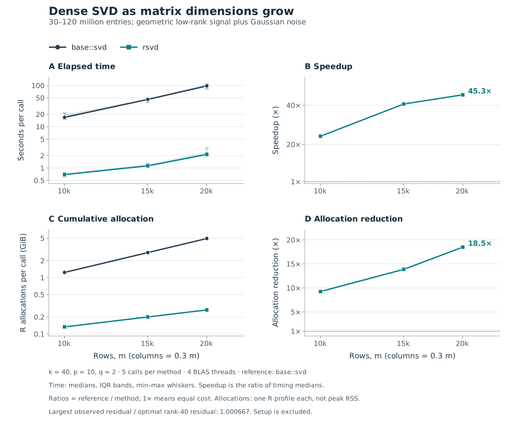
At 20,000 × 6,000, randomized SVD is 45.3× faster and reduces
cumulative R allocations by a factor of 18.5 relative to base SVD. The
relative errors are 9.68% and 9.67%, respectively, so most of the
residual comes from rank-40 truncation. The plot holds
k = 40 while input size grows from 30 million to 120
million entries. Shading gives the interquartile range of timings, and
whiskers show their minimum and maximum. Ratio panels use a 1× reference
line.
The largest dense input alone occupies about 0.89 GiB in double precision, before factorization workspace. Input size and the ratio of sketch width to input width affect the measured advantage. These results describe the stated inputs and numerical environment; speedup will vary with the matrix and the computation requested.
PCA adds preprocessing to the factorization. Both methods here center
and scale columns and return k = 40 loadings and score
columns. The reference is
prcomp(as.matrix(A), rank. = k, center = TRUE, scale. = TRUE).
Randomized PCA uses p = 10, q = 2. The sparse fixtures have
5% nonzero entries in twenty noisy blocks, and rpca()
applies their centering and scaling through sparse products.
The dense case gives a 10.3× speedup with both reconstruction errors rounding to 10.3%. For the largest sparse case, the speedup is 56.0×, with both errors rounding to 0.548%. The sparse comparison includes the cost of dense preprocessing in the reference.
| Input | k | Time (s) | Speedup | R allocations (GiB) | Relative error |
|---|---|---|---|---|---|
| Dense PCA, 15,000 × 4,500 | 40 | 54.085 / 5.256 | 10.3× | 8.056 / 2.981 | 10.3% / 10.3% |
| Sparse-input PCA, 10,000 × 3,000 | 40 | 18.336 / 0.463 | 39.6× | 3.806 / 0.213 | 0.516% / 0.516% |
| Sparse-input PCA, 20,000 × 6,000 | 40 | 110.634 / 1.976 | 56.0× | 15.212 / 0.482 | 0.548% / 0.548% |
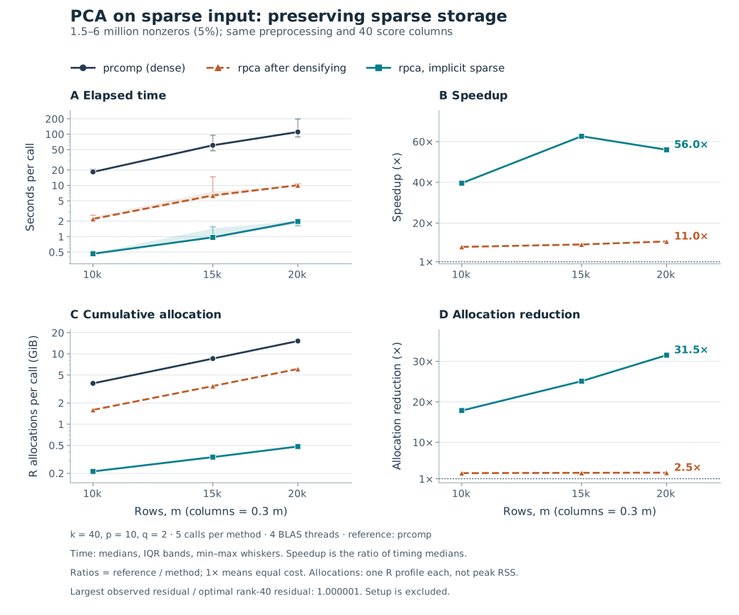
At the largest size, PCA with implicit sparse preprocessing is
56.0× faster and reduces cumulative R allocations by a factor of 31.5
relative to prcomp(). It is also 5.1× faster than
rpca(as.matrix(A), ...) on the same input. All three curves
use the same observations, preprocessing choices, and requested output.
The figure reports the maximum observed error relative to the optimal
rank-40 error.
The third curve keeps the randomized solver while changing whether
the input is densified. This comparison separates the benefit of
preserving sparse storage from the benefit of randomized factorization.
The speedup over prcomp() peaks at the middle size; runtime
variation and machine behavior mean it need not increase monotonically
with matrix dimensions.
Here PCA on sparse input produces ordinary principal components. The
loadings are generally dense, since rpca() does not impose
sparsity on them.
For ID and CUR, the deterministic references are
rid(rand = FALSE) and rcur(rand = FALSE),
which use LAPACK column-pivoted QR. Base R has no corresponding
functions. Both paths return the selected data subsets together with
their interpolation or connector factors. Randomized calls use
k = 40, p = 10, q = 0.
These subset approximations reduce computation while allowing their residuals to differ from the deterministic selections. For example, the dense column ID gives a 63.9× speedup, with relative error increasing from 14.3% to 15.8%. The sparse column ID gives a 163.5× speedup, and both errors round to 0.153%.
| Input | k | Time (s) | Speedup | R allocations (GiB) | Relative error |
|---|---|---|---|---|---|
| Column ID, dense, 15,000 × 4,500 | 40 | 43.727 / 0.684 | 63.9× | 1.257 / 0.326 | 14.3% / 15.8% |
| CUR, dense, 15,000 × 4,500 | 40 | 42.141 / 1.076 | 39.2× | 1.546 / 0.615 | 18.1% / 19.2% |
| Column ID, sparse, 15,000 × 4,500 | 40 | 46.938 / 0.287 | 163.5× | 1.522 / 0.095 | 0.153% / 0.153% |
| CUR, sparse, 15,000 × 4,500 | 40 | 40.352 / 0.346 | 116.6× | 1.572 / 0.145 | 0.189% / 0.189% |
Column-pivoted QR does not guarantee the optimal rank-k
approximation for every input. Reporting the residual beside time and
allocations shows the accuracy attained by each selection, including the
cases where the randomized result has a larger error.
The sparse PCA measurements depend on how preprocessing is carried out. Subtracting a nonzero mean from a sparse column turns its structural zeros into nonzero values. Storing the centered matrix explicitly would therefore usually require dense storage. Products with that matrix can instead be computed from the sparse input and a correction. For a vector of column means mu and a sketch matrix W,
(A-\mathbf{1}\mu^{T})W = AW-\mathbf{1}(\mu^{T}W).The vector 1 has an entry equal to one for each row
of A. The first term on the right uses a sparse product. The second
repeats the weighted column means across rows, giving the rank-one
centering correction. rpca() combines this identity with
implicit scaling to work with the processed observations. The sketches
and loadings are dense, but the full centered input need not be
stored.
set.seed(42)
# A 10,000 by 3,000 sparse matrix: 20 signal-plus-noise blocks, 5% density.
A <- Matrix::bdiag(replicate(20, {
  signal <- outer(seq_len(500) / 500, seq_len(150) / 150)
  signal + matrix(rnorm(500 * 150, sd = 0.001), 500, 150)
}, simplify = FALSE))
fit <- rpca(A, k = 20, center = TRUE, scale = TRUE, retx = FALSE)
scores <- predict(fit, A[1:5, , drop = FALSE])
An explicit k and rand = TRUE enable this
preprocessing for real sparse Matrix inputs. retx = FALSE
omits training scores and avoids computing unused left singular vectors.
Prediction applies the fitted transformation to new observations. Supply
their columns in the training order, since names are not used to reorder
them.
As in prcomp(), center = FALSE skips
centering. It can be used with data already centered by the caller or to
request an uncentered SVD. When centering is off,
scale = TRUE divides a real column by
sqrt(sum(x^2) / (nrow(A) - 1)), which generally differs
from its centered standard deviation. rpca() enables
scaling by default, whereas prcomp() leaves it off. The
existing rsvd convention replaces scales below 1e-8 with
1.
The returned fit$var accounts for all processed
observations, including variation outside the retained components. It is
their squared Frobenius norm divided by m - 1, where
m is the number of complete observations. With centering,
this equals the sum of all component variances, so explained proportions
use the same denominator for every k. Without centering, it
measures total squared energy with the same normalization. Sample
variances require at least two complete observations, and explained
proportions are undefined when the processed input has zero energy.
Fitted scores use the U D convention.
predict() instead projects observations onto the fitted
loadings, so prediction on the training data can differ from the stored
scores by the randomized approximation residual. This distinction
matters when comparing fitted coordinates with projections of new
observations.
The preprocessing choice is one part of the memory cost. The table summarizes where the algorithms preserve sparse input and where dense arrays are required.
| Routine | Sparse input and dense workspace |
|---|---|
rsvd(), randomized rqb() |
Keep sparse input for products; sketches, bases, and projected factors are generally dense. |
Randomized rid(), rcur() |
Use sparse sketch products and dense projected or selected factors. |
rpca(rand = TRUE, k = ...) |
Centers/scales real sparse input implicitly; loadings, sketches, and optional scores are dense. |
rpca(rand = FALSE) or rpca(k = NULL) |
Uses dense preprocessing and deterministic SVD. |
Deterministic rid(), rcur() |
Use dense pivoted QR, which can require a full dense copy. |
Deterministic rqb() |
Factors an independent real leading block when it reproduces the base-QR basis; otherwise falls back to full dense QR. |
rrpca() |
Uses dense input and dense working arrays. |
For ell = min(k + p, min(dim(A))), thin randomized
workspace scales with (nrow(A) + ncol(A)) * ell, in
addition to input storage and factorization workspace. Sparse
preprocessing also uses storage proportional to the stored entries. A
full reconstruction or residual matrix is dense even for sparse input,
so retaining factors can avoid that allocation.
rid(idx_only = TRUE) and
rcur(idx_only = TRUE) omit the selected data subsets from
the return value. They still compute the interpolation or connector
factors, which remain part of the calculation’s cost.
The preceding decompositions approximate the observed matrix
directly. Robust PCA instead models it as a low-rank component plus an
entrywise sparse corruption component. rrpca() seeks this
separation by minimizing a nuclear norm plus lambda times
an entrywise absolute sum. The nuclear norm is the sum of singular
values and encourages a low-rank component; the absolute-sum penalty
encourages sparsity in the corruption component.
Many candidate splits can reconstruct the same input closely, so a small reconstruction residual alone cannot establish that the objective has been minimized. The solver checks both reconstruction feasibility and stationarity. It expands saturated singular-value thresholding steps and refines stalled randomized updates, using an exact-SVD fallback when necessary.
maxiter limits the work and can stop the solver before
convergence. The returned err records reconstruction
errors; trace = TRUE also reports the stationarity
diagnostic. Stronger convergence checks can require more computation,
and the method retains dense working arrays. The release review describes
the optimality checks used in validation and what they establish.
R CMD build .
R CMD check --as-cran rsvd_2.0.0.tar.gz
With development dependencies installed,
testthat::test_local() runs the suite interactively. The
tests assess approximation against prescribed spectra, invariant
subspaces, complex arithmetic, and public result shapes. They also cover
sparse representations and implicit PCA products, rank-deficient ID and
CUR, and rank selection and convergence in robust PCA. CI verifies the
Matrix version before testing on Linux, Windows, and macOS, including R
4.4 with Matrix 1.7-0 at the supported minimum.
NEWS.md records the changes in 2.0.0, including compatibility and memory behavior. The November release review records the current corrections and validation. The earlier release review records the October numerical audit, downstream checks, tested environments, and their limitations. Its results apply to the source revisions named there. The benchmark guide and measurements provide the scripts and data for reproducing the tables and figures or evaluating matrices representative of another workload.
@Article{,
  title = {Randomized Matrix Decompositions Using {R}},
  author = {N. Benjamin Erichson and Sergey Voronin and Steven L.
    Brunton and J. Nathan Kutz},
  journal = {Journal of Statistical Software},
  year = {2019},
  volume = {89},
  number = {11},
  pages = {1--48},
  doi = {10.18637/jss.v089.i11},
}