


rasch fits and evaluates models within Rasch Measurement
Theory. It includes models for item responses, explanatory item and
threshold structures, multiple ratings, linked frames of reference, and
paired comparisons, with a common set of functions for examining fit,
invariance, targeting, dimensionality, and local dependence.
The original dichotomous model is (Rasch, 1960)
\[ \log\frac{P(X_{ni}=1)}{P(X_{ni}=0)}=\theta_n-\delta_i, \]
which is distinguished among item response models by its sufficiency and invariance properties: the total score is sufficient for the person parameter, so items can be compared independently of the persons who responded. This sufficiency allows item locations to be estimated by pairwise conditioning (Zwinderman, 1995): given exactly one of items \(i\) and \(j\) correct, the person parameter cancels,
\[ \log\frac{P(X_{ni}=1 \mid X_{ni}+X_{nj}=1)}{P(X_{nj}=1 \mid X_{ni}+X_{nj}=1)}=\delta_j-\delta_i, \]
which is equivalent to the standard model for comparative judgement (Andrich, 1978a; Bradley and Terry, 1952; Luce, 1959). The extensions keep this structure: partial credit and rating scale models add ordered thresholds (Andrich, 1978b; Masters, 1982); the many-facet model adds rater and task locations to the composite (Linacre, 1989); the extended frame of reference model links frames measured in different units (Humphry and Andrich, 2008); polytomous comparative judgement applies the thresholds to ordered pair judgements (Tutz, 1986). The linear logistic test model and linear partial credit model express item or threshold locations as functions of observed characteristics (Fischer, 1973; Fischer and Ponocny, 1994). The same explanatory formulation can be applied to object locations in dichotomous or ordered comparative judgements.
The package treats fit to the model as an empirical question. Its diagnostics examine whether comparisons remain invariant across persons, items, groups, occasions, raters, and other parts of the measurement design.
| Function | Model |
|---|---|
rasch() |
Dichotomous Rasch, partial credit, and rating scale models |
rasch_mfrm() |
Many-facet Rasch model |
rasch_efrm() |
Extended frame of reference model |
rasch_explanatory() |
Linear logistic test and linear partial credit models |
btl() |
Comparative judgement models for dichotomous and polytomous paired comparisons |
btl_efrm() |
Extended frame of reference model for paired comparisons |
btl_explanatory() |
Explanatory comparative judgement models |
Person measures are estimated by weighted likelihood (Warm, 1989). Externally imposed item or item-set weights can be used for a supplementary person measure without changing the fitted calibration or its diagnostics. Anchored estimation is available for equating, and incomplete linked designs can be fitted when their observed response structure identifies a common scale.
The item-response models follow Rasch (1960) and Andrich and Marais (2019). The explanatory item models follow Fischer (1973) and Fischer and Ponocny (1994), within the explanatory framework of De Boeck and Wilson (2004). Continuous, categorical or ordinal characteristics may be used; the comparative-judgement formulation applies the same fixed design to Bradley–Terry–Luce object locations. The frame models follow Humphry (2005) and Humphry and Andrich (2008). The comparative judgement models follow Bradley and Terry (1952), Luce (1959), Andrich (1978a), and Tutz (1986).
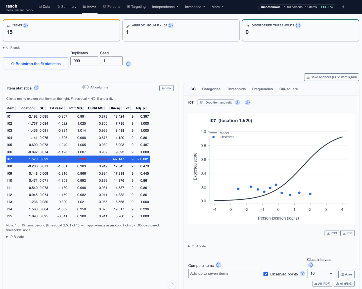
The package includes a graphical interface for analysts who do not normally work in R. Launch it after installation with:
rasch::run_app()The application imports data, assigns variables to their measurement
roles, fits the selected model, and displays the resulting tables and
plots. An analysis can be saved as a .rasch project and
reopened with its data roles and estimation settings. Tables, figures
and HTML, Word or PDF reports can be downloaded. The R code for each
result is shown in the interface. Its fit bootstrap calibrates item and
person fit, or pair, object and judge fit for comparative judgement, in
a cancellable background process. Its adjusted probabilities refer to
the fitted global null, separately for each statistic. The simulation
page generates each supported data structure, with controls for its
principal parameters and planted departures. Simulated data can be
downloaded as a CSV or together with the generating call, true values
and explanatory metadata.
Install the CRAN release with:
install.packages("rasch")The development version is available from GitHub:
# install.packages("remotes")
remotes::install_github("drjoshmcgrane/rasch")library(rasch)
d <- simulate_rasch(
n_persons = 500,
n_items = 10,
n_groups = 2,
seed = 1
)
fit <- rasch(d, model = "PCM", id = "id", factors = "group")
summary(fit)
fit_summary_table(fit)
targeting_table(fit)
dif <- dif_anova(fit)
residual_correlations(fit)
dimensionality_test(fit, B = 99, seed = 1)
# Optional sensitivity analysis for the DIF reference distribution
dif_bootstrap(fit, dif, B = 999, seed = 1)
# Calibrated item and person fit (use more replicates for a final analysis)
boot <- fit_bootstrap(fit, B = 199, seed = 1)
boot$items
boot$persons
plot_pimap(fit)
plot_icc(fit, "I05", group = "group")
# WrightMap is an optional dependency
wright_map(fit, person_panels = "group")The DIF bootstrap is a sensitivity analysis under the fitted global invariant null. The adjusted residual analysis remains primary.
The function reference documents the data requirements and returned values for each analysis. The vignettes begin with the data structures required by each model and cover the Rasch workflow, many-facet and extended-frame models, comparative judgement, explanatory modelling, repeated-measures DIF and validation.
Andrich, D. (1978a). Relationships between the Thurstone and Rasch approaches to item scaling. Applied Psychological Measurement, 2(3), 451–462.
Andrich, D. (1978b). A rating formulation for ordered response categories. Psychometrika, 43(4), 561–573.
Andrich, D., and Marais, I. (2019). A Course in Rasch Measurement Theory: Measuring in the Educational, Social and Health Sciences. Springer.
Bradley, R. A., and Terry, M. E. (1952). Rank analysis of incomplete block designs: I. The method of paired comparisons. Biometrika, 39(3/4), 324–345.
De Boeck, P., and Wilson, M. (Eds.). (2004). Explanatory Item Response Models: A Generalized Linear and Nonlinear Approach. Springer.
Fischer, G. H. (1973). The linear logistic test model as an instrument in educational research. Acta Psychologica, 37(6), 359–374.
Fischer, G. H., and Ponocny, I. (1994). An extension of the partial credit model with an application to the measurement of change. Psychometrika, 59(2), 177–192.
Humphry, S. M. (2005). Maintaining a Common Arbitrary Unit in Social Measurement. PhD thesis, Murdoch University.
Humphry, S. M., and Andrich, D. (2008). Understanding the unit in the Rasch model. Journal of Applied Measurement, 9(3), 249–264.
Linacre, J. M. (1989). Many-Facet Rasch Measurement. MESA Press.
Luce, R. D. (1959). Individual Choice Behavior: A Theoretical Analysis. Wiley.
Masters, G. N. (1982). A partial credit model for scoring responses with ordered categories. Psychometrika, 47(2), 149–174.
Rasch, G. (1960). Probabilistic Models for Some Intelligence and Attainment Tests. Danish Institute for Educational Research. Expanded edition, University of Chicago Press, 1980.
Tutz, G. (1986). Bradley-Terry-Luce models with an ordered response. Journal of Mathematical Psychology, 30(3), 306–316.
Warm, T. A. (1989). Weighted likelihood estimation of ability in item response theory. Psychometrika, 54(3), 427–450.
Zwinderman, A. H. (1995). Pairwise parameter estimation in Rasch models. Applied Psychological Measurement, 19(4), 369–375.
Use citation("rasch") to obtain the citation for the
installed version.